Configuring Tag History
In 8.1.17, the Tag Editor was redesigned to improve usability. The new Tag Editor now requires fewer clicks and keeps relevant tag information visible while modifying bindings, alarms, and event scripts.
Pages detailing features of the previous Tag Editor can be found in Deprecated Ignition Features.
Logging data is easy with Tag Historian. Once you have a database connection, all you do is set the tags to store history and Ignition takes care of the work. Ignition creates the tables, logs the data, and maintains the database.
The historical tag values pass through the store-and-forward engine before ultimately being stored in the database connection associated with the historian provider. The data is stored according to its data type directly to a table in the SQL database, along with its quality and a millisecond resolution timestamp. The data is only stored on-change, according to the value mode and deadband settings on each tag, thereby avoiding duplicate and unnecessary data storage. The storage of Tag Group execution statistics ensures the integrity of the data.
The first step to storing historical data is to configure tags to record values. This is done from the History section of the Tag Editor in the Designer. Select the History Enabled property to turn on history. The properties include an Historical Tag Group that will be used to check for new values. Once values surpass the specified deadband, they are reported to the history system, which then places them in the proper store and forward engine.
Enable History on a Tag
The following example demonstrates how to configure a tag to store values into the Tag Historian. Complete information on the History properties (and all properties in the Tag Editor), can be found on the Tag Properties Table.
Dataset type tags are not supported by the Tag History system.
-
In the Tag Browser, select one or more tags. For example, we selected several Sine tags in the Sine folder.
-
Right-click on the selected tags, and then select Edit Tag
 . The Tag Editor window is displayed where you can change the tag name, data type, scaling options, metadata, permissions, history, and alarming.
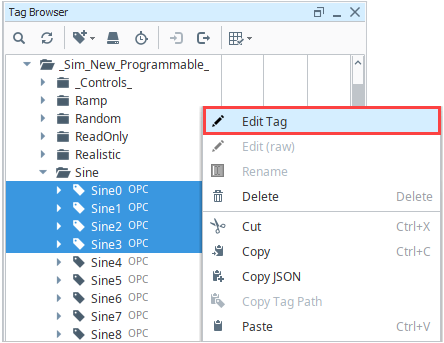
-
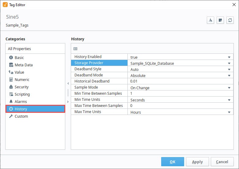
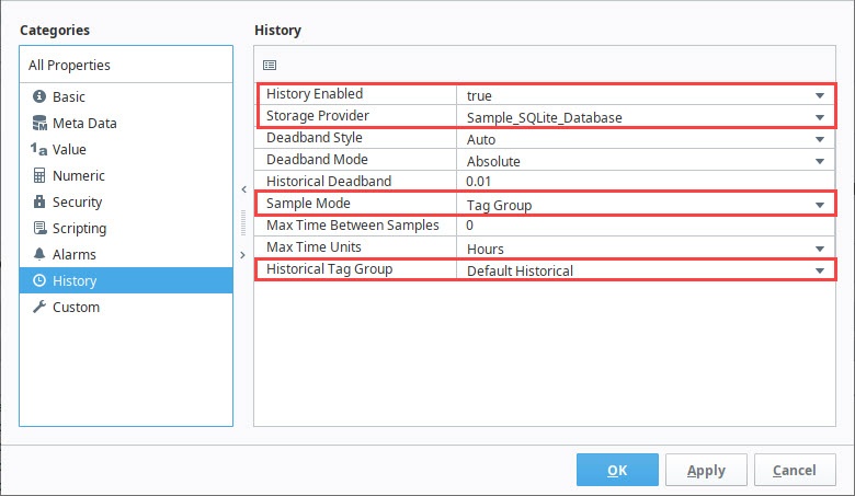
Scroll down to History or select the History pane on the Tag Editor. Set History Enabled to true.
-
Choose a database (for example, SQLite) from the Storage Provider dropdown.
-
Set the Sample Mode to Tag Group.
-
Set the Historical Tag Group to Default Historical.
-
Click OK. Now look in the Tag Browser. To the right of each Sine tag that is storing history, a History
 icon appears letting you know it is set up.
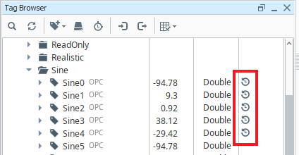
Now, if you look in your database, you can see all the tables and data Ignition has created for you.
Setting a UDT to Log History Data
Enabling tag history on members in a UDT involves editing the UDT definition, and enabling history on the any members you wish to record. These history settings will then propagate to members in any instances.
Tag History Configuration
Below is a description of some important tag history settings.
Sample Mode
The Sample Mode setting determines how often the Tag History system will check if the tag’s value should be stored to the database using Deadband and Deadband Style settings.
- On Change - Ignition will check if the value should be stored to the database each time the tag value changes.
- Periodic - Ignition will check if the value should be stored to the database at a specific rate defined by the Sample Rate property.
- Tag Group - Ignition will check if the value should be stored to the database at the specific rate defined within the Tag Group selected under the Historical Tag Group property.
Historical Tag Group
The Historical Tag Group setting is visible when Sample Mode is set to Tag Group. The Historical Tag Group setting determines how often to check if the value on the tag should be stored. It uses the same Tag Groups that dictate how often your tags should execute. Typically, the Historical Tag Group should execute at the same rate as the tag's Tag Group or slower. For example, if a tag's Tag Group is set to update at a 1,000ms rate, but the Historical Tag Group is set to a Tag Group that runs at 500ms rate, then the Tag History system will be checking the tag's value twice between normal value changes, which is unnecessary.
Max and Min Time Between Samples
Normally, Tag Historian only stores records when values change. By default, an "unlimited" amount of time can pass between records – if the value doesn't change, a new row is never inserted in the database. By modifying these settings, it is possible to specify the maximum number of Tag Group execution cycles that can occur before a value is recorded. Setting the value to 1, for example, would cause the tag value to be inserted each execution, even if it has not changed. Given the amount of extra data in the database that this would lead to, it's important to only change this property when necessary.
The Max Time Between Samples property cannot be less than 1000ms.
Interpolated Values
When the Ignition historian queries a database for historical data, there may be intervals with no raw data in the database. When this happens, Ignition interpolates the missing data. Interpolation is the process of estimating unknown values that fall between known values, and is calculated depending on the tag configuration or selected Aggregation Mode, as long as AvoidInterpolation is false. Although interpolated values are calculated every time a raw data point is found or when an interval ends based on the configuration or Aggregation Mode selections, the values are reserved to be used only when there are no data points in an interval.
To demonstrate how interpolation works, example data queried using a traditional Tag History binding from 1:30pm to 5:30pm in 60 minute time windows is shown below. The query returned three windows with data and one window with no data.
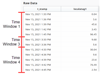
- Time Window 1 - 1:30pm through 2:30pm: 0.04, 5.6, 45.6, 3.45, 96.45
- Time Window 2 - 2:30pm through 3:30pm: no data in this time window
- Time Window 3 - 3:30pm through 4:40pm: 9.68, 5.6
- Time Window 4 - 4:30pm through 5:30pm: 30.04, 9.6, 23.6, 76.49, 2.54
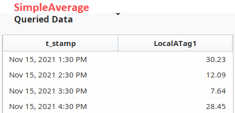
If you select SimpleAverage as your Aggregation Mode, the request returns a row representing the SimpleAverage value for every time window. The value in the first row was calculated by averaging all of the values between 1:30pm - 2:30pm:
(0.04 + 5.6 + 45.6 + 3.45 + 96.45) / 5 = 30.23
This same method applies to the third and fourth row values. However, since there are no raw records between 2:30pm - 3:30pm, the value of 12.09 is calculated using interpolation.
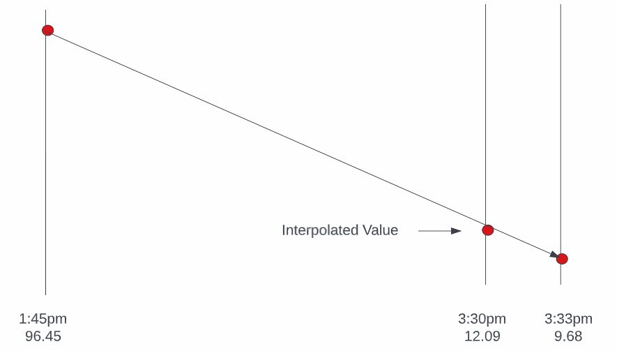
12.09 was obtained by marking the end point of the empty window along a line connecting the last value from the previous window to the first value in the next window. This is easily shown using a chart to visualize where the time and value intersect. The last value in the previous time window is marked at 96.45 and the first value in the next time window is marked at 9.68. Once the line is drawn between the two, the marked value at the end of the empty window end time (3:30pm) gives us the interpolated value of 12.09.
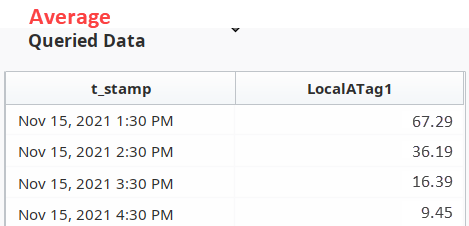
The interpolated value remains 12.09 for every Aggregation Mode we query for unless we select the Average Aggregation Mode, which returns a value of 36.19.
The Average Aggregation Mode is an exception to the previously described interpolation method because the time-weighted calculation included in the Average process remains the same whether there are or aren't data points in a time interval.
The time-weighted process uses current and previous values with the interval time difference in milliseconds to determine Average values.
- Average Value = (0.5 * abs((currVal - prevVal) * timediff)) + (timediff)(min(currVal,prevVal))
If we use the same data from the earlier example, the process looks like:
prevVal = 96.45
currVal = 60.29
Since the current value, or end time of the first window, has no data the value is obtained with a retValue process. The required data for this process includes the last value in the previous non-empty window, represented by A; the first value in the next non-empty window, represented by B; and the amount of time between the last value in the previous non-empty window divided by the total time between collected values.
- retValue = A + ((B-A) * ((ts - Ats) / (Bts - Ats)))
A = 96.45
B = 9.68
Bts - Ats = 3:33pm - 1:45pm > 108 minutes
ts - Ats = 2:30pm - 1:45pm > 45 minutes

96.45 + ((9.68 - 96.45) (45/108)) = 60.29
If there was data for the 2:30pm interval, which is the end of Time Window 1, that would be used as the current value and no further calculations would be required.
Since the previous value was collected at 1:45pm and the current value was collected at 2:30pm, the time difference is 45 minutes. Since time difference is calculated in milliseconds, 2,699,999 is used:
timediff = 2,699,999
Therefore the process calculation for the first window is:
(0.5 * abs((60.2958 - 96.45) * 2,699,999)) + (2,699,999)(min(60.2958)) = 211,606,751.6271
Add this result to the sum of all Average values for the data between 1:33pm and 1:45pm to include all time-weighted data.
The same process calculation is used for the values between 1:33pm and 1:45 as used for the first window calculation above.
Time        Value
1:33        0.04
1:36        5.6
1:39        45.6
1:42        3.45
1:45        96.45

1:33 to 1:36:
(0.5 * abs((5.6-0.04) * 179,999)) + 179,999(0.04) = 507,597.18

1:36 to 1:39:
(0.5 * abs((45.6-5.6) * 179,999)) + 179,999(5.6) = 4,607,974.4

1:39 to 1:42:
(0.5 * abs((3.45-45.6) * 179,999)) + 179,999(3.45) = 4,414,475.47

1:42 to 1:45:
(0.5 * abs((96.45-3.45) * 179,999)) + 179,999(3.45) = 8,990,950.05

507,597.18 + 4,607,974.4 + 4,414,475.47 + 8,990,950.05 = 18,520,997.1
Then, divide by the total time that has passed, which is 57 minutes (1:33pm-2:30pm) or 3,419,999ms:
(211,606,751.6271 + 18,520,997.1) / 3,419,999 = 67.29
As shown in the queried values above, 67.29 is the Average value for Time Window 1.
Now, instead of just creating a chart to find the linear interpolated value and moving on, we must follow the same Average process for the empty window to apply the time-weighted calculations. To do this, we will still use the linear interpolated value of 12.09 as the current value in the process since the window has no data. The current value of 60.29 used in the Time Window 1 process becomes the previous value for this Time Window 2 process.
prevVal = 60.29
currVal = 12.09
Since the time window interval is from 2:30pm to 3:30pm, we use 60 minutes, or 3599999ms for the time difference:
timediff = 3599999
Therefore, the process calculation for the empty window is:
(0.5 * abs((12.09 - 60.2958) * 3,599,999)) + (3,599,999)(min(12.09)) = 130,283,963.81
Lastly, to get the Average interpolated value this number is divided by the total time that has passed, which is 60 minutes or 3,599,999ms:
130,283,963.81 / 3,599,999 = 36.19
Deadband Discrete Style and Analog Compression
This section describes the Deadband Style property options Auto, Analog, and Discrete because it may not be immediately clear how the deadband value is used differently depending on whether the tag is configured as a Discrete tag or as an Analog tag. Discrete values are more straightforward, registering a change any time the value moves +/- the specified amount from the last stored value. However, with Analog tags the deadband value is used more as a compression threshold, in an algorithm similar to that employed in other Historian packages. It is a modified version of the 'Sliding Window' algorithm. The following examples show the process in action, comparing a raw value trend to a "compressed" trend.
Discrete
Storage: The deadband will be applied directly to the value. That is, a new value (V1) will only be stored when: |V1-V0| >= Deadband.
Interpolation: The value will not be interpolated. The value returned will be the previous known value, up until the point at which the next value was recorded.
Analog
Storage: Every time the tag's value changes, this method will calculate upper and lower slope values. These slope values are stored in memory, and are ultimately used to determine when a new value is stored. The calculations used are listed below:
(((NewValue + Deadband) - PreviousValue) / (NewTimestamp - PreviousTimestamp))
(((NewValue - Deadband) - PreviousValue) / (NewTimestamp - PreviousTimestamp))
The algorithm will only store new values under the following conditions:
- The system always stores the first value on the tag when using the method, since the subsequent values will need an initial value to calculate slope from.
- If the newly calculated upper slope is lesser than the previously calculated lower slope value, the system will store the new value.
- If the newly calculated lower slope is greater than the previously calculated upper slope value, the system will store the new value.
- The system always stores a value when the quality on the tag changes.
In cases where a new value isn't stored, the system will compare the newly calculated slope values to the previously calculated values:
- If the new upper slope is less than the previous upper slope, then the new upper slope is used for future comparisons.
- If the new lower slope is greater than the previous lower slope, then the new lower slope is used for future comparisons.
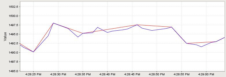
In the image below, an analog value has been stored. The graph has been zoomed in to show detail; the value changes often and ranges over time +/- 10 points from around 1490.0. The compressed value was stored using a deadband value of 1.0, which is only about .06% of the raw value, or about 5% of the effective range. The raw value was stored using the Analog mode, but with a deadband of 0.0. While not exactly pertinent to the explanation of the algorithm, it is worth noting that the data size of the compressed value, in this instance, was 54% less than that of the raw value.
Interpolation: The value will be interpolated linearly between the last stored value and the next value. For example, if the value at Time0 was 1, and the value at Time2 is 3, selecting Time1 will return 2.
Auto
This setting will automatically pick either Analog or Discrete, based on the data type of the tag. Auto is the default Deadband Style when initially configuring tag history.
- If the data type of the tag is set to a float or double, then Auto will use the Analog Style.
- If the data type of the tag is any other type, then the Discrete style will be used.
Example
Let's look at a demonstration of how the analog compression works. For this example we'll assume a tag is using a historical deadband value of 0.01. Over the course of a few moments the tag's value changed several times, as represented on the chart below.
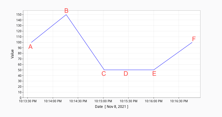
The tag historian system stores the records into one of the data partitions. After the value changes above, our database stores the records.
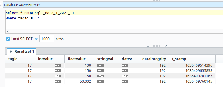
Below we'll describe how each value was stored as the tag changed value.
Value A
Once we enable history on the tag and set the deadband style to Analog, the system will record the first value on the tag. Since we only have a single value, the system uses arbitrarily large and small placeholder values for the slope envelope (3.40282347 x 10^38 and -3.40282347 x 10^38, respectively) until the tag changes again.
Value B
Now the tag changes to 150. Since this is only the second value observed, the system calculates slope values for the first time using the formula listed above.
// Upper Slope
((150 + 0.01) - 100) / (1636409655838 - 1636409614396)
(150.01 - 100) / 41442
50.01 / 41442
0.001206768

// Lower Slope
((150 - 0.01) - 100) / (1636409655838 - 1636409614396)
(149.99 - 100) / 41442
49.99 / 41442
0.0012062641
Because the original slope placeholders were temporary, the system replaces them with these new values. However, the new tag value 150 is not stored yet, but is held in memory until the next value comes in.
Value C
The tag changes again, this time to 50. The system calculates new slope values using 150 as the previous value.
// Upper Slope
((50 + 0.01) - 150) / (1636409701167 - 1636409655838)
(50.01 - 150) / 45329
-99.99 / 45329
-0.0022058727

// Lower Slope
((50 - 0.01) - 150) / (1636409701167 - 1636409655838)
(49.99 - 150) / 45329
-100.01 / 45329
-0.002206314
These new values meet our storage criteria:
- The new upper slope (-0.0022058727) is less than the previous lower slope (0.0012062641).
So the system stores the previous value (150) and adopts these new slope values to evaluate the next tag change. The new value of 50 is held in memory, waiting to be stored.
Value D
The tag changes to 50.001 after the system recalculates slope values using the last value of 50.
// Upper Slope
((50.001 + 0.01) - 50) / (1636409726809 - 1636409701167)
(50.011 - 50) / 25642
0.011 / 25642
4.289837E-7

// Lower Slope
((50.001 - 0.01) - 50) / (1636409726809 - 1636409701167)
(49.991 - 50) / 25642
-0.009 / 25642
-3.5098665E-7
These new slope values meet the storage condition:
- The new lower slope (-3.5098665E-7) is greater than the previous upper slope (-0.0022058727).
So the system stores the previous value (50) and adopts the new slope values. The current value (50.001) is held in memory for now.
Value E
Now the tag changes to 50.002. New slope values are calculated using the previous value of 50.001.
 // Upper Slope
 ((50.002 + 0.01) - 50.001) / (1636409760145 - 1636409726809)
 (50.012 - 50.001) / 33336
 0.011 / 33336
 3.300870E-7

 // Lower Slope
 ((50.002 - 0.01) - 50.001) / (1636409760145 - 1636409726809)
 (49.992 - 50.001) / 33336
 -0.009 / 33336
 -2.700713E-7
These values do not meet storage criteria:
- The new upper slope (3.300870E-7) is not less than the previous lower slope (-3.5098665E-7).
- The new lower slope (-2.700713E-7) is not greater than the previous upper slope (4.289837E-7).
So, the system does not store 50.001, and holds on to 50.002 in memory. However, the system notices that the slope envelope has become more restrictive:
- The new upper slope is smaller than the previous upper slope
- The new lower slope is larger than the previous lower slope
Since both bounds have tightened, the system updates the envelope to use these new slope values. They’ll be used the next time the tag value changes to determine whether storage is necessary.
Value F
The tag jumps to 100. Slope values are calculated using the previous value 50.002.
// Upper Slope
((100 + 0.01) - 50.002) / (1636409786810 - 1636409760145)
(100.01 - 50.002) / 26665
50.008 / 26665
0.0018754172

// Lower Slope
((100 - 0.01) - 50.002) / (1636409786810 - 1636409760145)
(99.99 - 50.002) / 26665
49.988 / 26665
0.0018746671
These slope values meet the storage condition:
- The new lower slope (0.0018746671) is larger than the previous upper slope (3.300870E-7).
Because this condition is satisfied, the system stores the previous value (50.002) and updates the slope envelope with the newly calculated values.
This process continues as the tag value changes over time, with the slope window dynamically adjusting based on how different each new value is.
In addition to the Deadband Style, your tag history settings also include the Deadband Mode and Historical Deadband properties.
- Deadband Mode is set to Absolute by default. If changed to Percent, the deadband is calculated as a percentage of the tag’s engineering unit span.
- Historical Deadband applies specifically to historical data evaluation.
- If Deadband Mode is set to Off, all values are stored when the timestamp changes.
Seeded Values
Tag history queries sometimes use seeded values (occasionally called "Boundary Values"). When retrieving tag history data, the system will also retrieve values just outside of the query range (before the start time, after the end time), and include them in the returned result set. They're generally used for interpolation purposes. If you do not want to include these seeded values, interpolation must not be enabled. The following is also required:
- Have the tag store history with a Discrete Mode
- Set the [noInterpolation] parameter to true
- Set the [includeBoundingValues] parameter to false on the calling query
Pre-Query Seed Value
These are a single value taken from just before the start of the query range. The value and timestamp for this value is typically the first row in the resulting query. Pre-query seed values are always included when not using a raw data query.
An exception to this rule is can be found with the system.tag.queryTagHistory function. Setting includingBoundingValues argument to True and returnSize to -1 will return a raw data query with a pre-query seed value.
Post-Query Seed Value
These extra values are added to the end of the result set, representing the next data point after the query range. Post-query seed values are only included when interpolation is requested/enabled for the query. Thus, values stored with a Discrete deadband style will not include post-query seed values in the query results, but an Analog deadband style will include post-query seed values.
If the system knows the query is retrieving records for a tag on the local system, this value will be determined by the current tag's value instead of retrieving the last recorded value in the database. The current tag's value is also used in cases where the time range extends to the present time.
If a result in a query is outside of the requested range, the value is typically a seeded value. This typically occurs when the range is so small that values were not recorded, or when the range is in the future (and thus values have not yet been recorded).
Raw Data Queries
In most cases, queries returned by tag history will apply some form of aggregation. However, it is possible to get a "raw data query", which is a result set that contains only values that were recorded: meaning no aggregation or interpolation is applied to the results. A raw data query can be obtained by using one of the following options:
- Set the Sample Size on Vision Tag History bindings to On Change
- Setting the returnSize parameter on system.tag.queryTagHistory or system.tag.queryTagCalculations to -1.
Be aware that if a tag is storing history using the Analog style, the returned dataset will include post-query seed values.
- Setting the Query Mode on Perspective Tag History bindings to AsStored